RLC Circuit Simulation
This document describes the implementation of an RLC circuit using pyams.lib for transient analysis. The simulation evaluates the voltage and current characteristics over time.
RLC Circuit
The RLC circuit consists of a resistor, inductor, and capacitor connected in series with a DC voltage source.
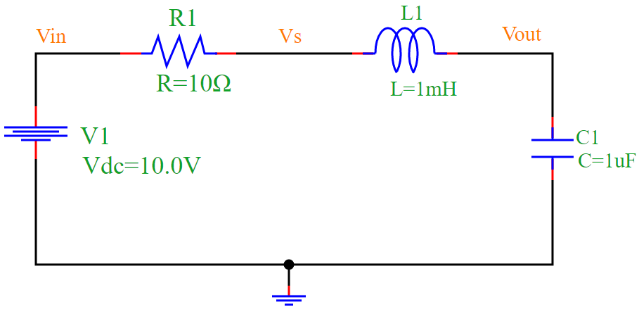
Figure 1: RLC Circuit Diagram.
The governing equation for an RLC circuit is:
Where:
\(V_R = i R\)
\(V_L = L \frac{di}{dt}\)
\(V_C = \frac{1}{C} \int i dt\)
Solving the Differential Equation
The second-order differential equation governing the circuit is:
For a step input (DC voltage \(V = V_0\)), the homogeneous solution is:
where \(s_1\) and \(s_2\) are the roots of the characteristic equation:
The roots determine the system response:
Overdamped: \(R^2 > 4L/C\), distinct real roots.
Critically damped: \(R^2 = 4L/C\), repeated real root.
Underdamped: \(R^2 < 4L/C\), complex conjugate roots leading to oscillations.
For the underdamped case, the solution takes the form:
where:
\(\alpha = \frac{R}{2L}\)
\(\omega_d = \sqrt{\frac{1}{LC} - \alpha^2}\)
Numerical Application
Given the circuit parameters:
\(R = 10 \Omega\)
\(L = 1 \text{mH} = 1 \times 10^{-3} \text{H}\)
\(C = 1 \text{μF} = 1 \times 10^{-6} \text{F}\)
\(V_0 = 10V\)
We calculate:
Damping coefficient:
\[\alpha = \frac{R}{2L} = \frac{10}{2 \times 10^{-3}} = 5000 \text{ s}^{-1}\]Resonant frequency:
\[ \begin{align}\begin{aligned}\omega_0 = \frac{1}{\sqrt{LC}} = \frac{1}{\sqrt{(1 \times 10^{-3}) (1 \times 10^{-6})}}\\\omega_0 = 10^6 \text{ rad/s}\end{aligned}\end{align} \]Damped frequency:
\[ \begin{align}\begin{aligned}\omega_d = \sqrt{\omega_0^2 - \alpha^2} = \sqrt{(10^6)^2 - (5000)^2}\\\omega_d \approx 999987.5 \text{ rad/s}\end{aligned}\end{align} \]
Since \(\alpha^2 \ll \omega_0^2\), the circuit is underdamped and exhibits oscillations.
Simulation Results
The transient response of the RLC circuit is obtained using the Python script below. The results show the voltage across the capacitor (Vout) and the current through the resistor (R1.I).
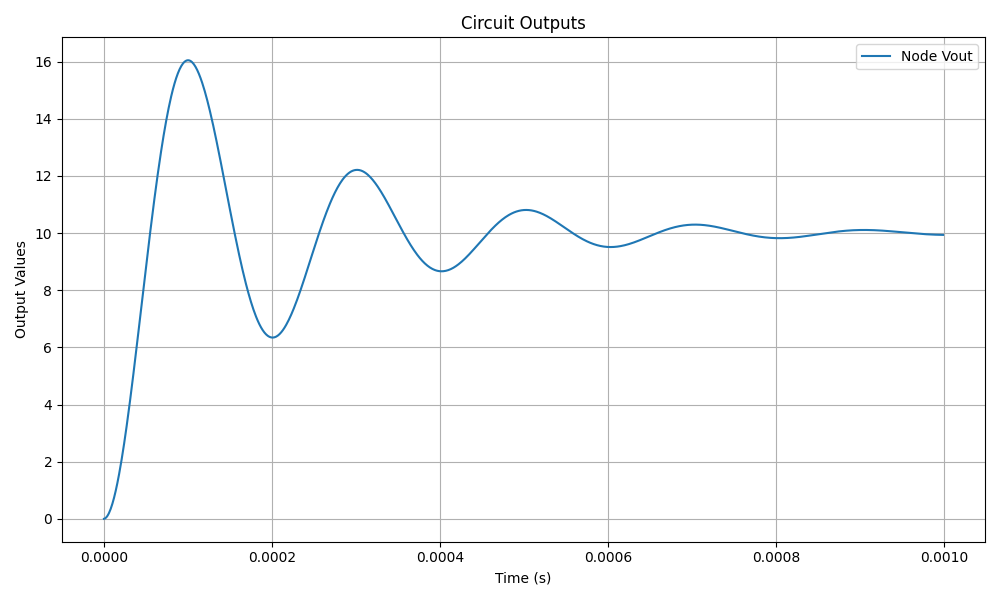
Figure 2: Voltage Output (Vout) of the RLC circuit.
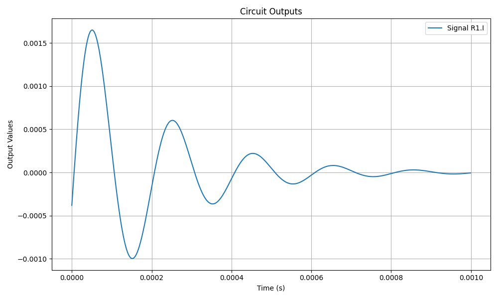
Figure 3: Current through Resistor (R1.I) in the RLC circuit.
Conclusion
The simulation successfully analyzes the transient response of an RLC circuit. The plotted results illustrate the characteristic oscillatory behavior of the circuit.